MISST - Microstructure Imaging Sequence Simulation ToolBox

Introduction

Microstructure Imaging Sequence Simulation Toolbox (MISST) is a practical diffusion MRI simulator for development, testing, and optimisation of novel MR pulse sequences for microstructure imaging. MISST is based on a matrix method approach and simulates the signal for a large variety of pulse sequences and tissue models. Its key purpose is to provide a deep understanding of the restricted diffusion MRI signal for a wide range of realistic, fully flexible scanner acquisition protocols, in practical computational time.

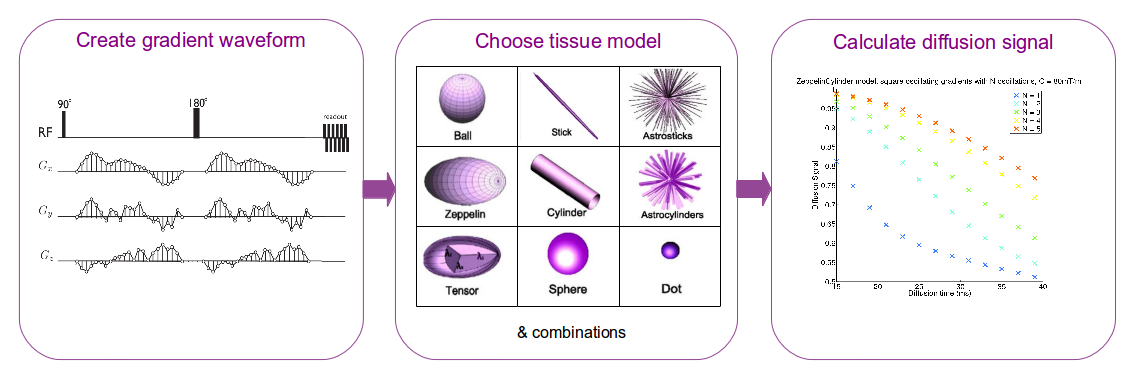
The novelty of MISST is that it simulates diffusion MRI signal with any user-defined diffusion gradient sequence from a standard PGSE to more advanced sequences such as oscillating gradients, dPFG, q-mas, STEAM, etc. The diffusion signal is calculated using the matrix formalism ( Callaghan 1997 ) and the implementation detailed in Drobnjak et al. 2010 and Drobnjak et al. 2011. The existing parametrizations for square and trapezoidal oscillating gradients follow the description in Ianus et al. 2012. The diffusion substrates available in MISST are the basic compartments presented in Panagiotaki et al. 2012, as well as some two- and three-compartment models of white matter.

Target audience

MISST is designed for diffusion MRI researchers who are interested in understanding and developing diffusion pulse sequences for imaging microstructure.

Download

Terms and Conditions

MISST is distributed under the Artistic License 2.0. The full text of the license can be found here . The Owner draws your attention to the fact that the Software has been developed solely for and is intended for use in a research environment ONLY. No endorsement can be given for other use including, but not limited to, use in a clinical environment. Compliance with this notice constitutes part of the license agreement.

If you are using MISST in your research, please cite Drobnjak et al. 2010 , Drobnjak et al. 2011, Ianus et al. 2012 and Ianus et al. 2016

Download MISST, release version 0.93 hosted on the NITRC website. By clicking this link you agree to the above Terms and Conditions

Documentation

Step-by-step getting started tutorial

Include MISST toolbox in the MATLAB search path:

Assuming that you have unpacked the MISST toolbox in the directory /usr/local/MISST, then run

addpath(genpath('/usr/local/MISST'))

You have to do this every time you open a new MATLAB session.

Example 1: square oscillating gradients
Create an example protocol with square oscillating gradients

We provide the means of generating the discrete gradient waveform for several parametrized sequences by calling the wave_form function. The available sequences are:

* pulse gradient spin echo sequence (PGSE)

* sinusoidal oscillating gradients (OGSE)

* square oscillating gradients (SWOGSE)

* trapezoidal oscillating gradients (TWOGSE)

* square oscillating gradients with different parameters in x,y and z directions (SWOGSE_3D)

* double pulsed field gradients (dPFG)

* stimulated echo sequences (STEAM)

* helical gradients (Helical)

If your sequence is not in this list you need to create it your self, see example 2 for guidance.

Detailed explanations are in the documentation.

Here we show an example for SWOGSE:

* Setup an initial protocol which includes the necessary information to compute the discrete waveform for a SWOGSE sequence

 % add some combinations of parameters:
clear all
delta = 0.015:0.005:0.04; % duration in s
smalldel = delta - 0.005;  % duration in s
Nosc = 1:5;  % number of lobes in the oscillating gradient. A full period has 2 lobes
G = 0.08; % gradient strength in T/m;
tau = 1E-4; % time interval for waveform discretization
it = 0;
protocol_init.pulseseq = 'SWOGSE';
for i = 1:length(delta)
    for j = 1:length(Nosc)
        it = it+1;
        protocol_init.smalldel(it) = smalldel(i);
        protocol_init.delta(it) = delta(i);
        protocol_init.omega(it) = Nosc(j).*pi./smalldel(i);
        protocol_init.G(it) = G;
        protocol_init.grad_dirs(it,:) = [1 0 0]; % gradient in x direction
    end
end
protocol_init.tau = tau;

* Create the GEN protocol (format required for the simulation)

protocolGEN.pulseseq = 'GEN';
protocolGEN.G = wave_form(protocol_init);
protocolGEN.tau = tau;
% include smalldel and delta as they make computation slightly faster
protocolGEN.delta = protocol_init.delta;
protocolGEN.smalldel = protocol_init.smalldel;

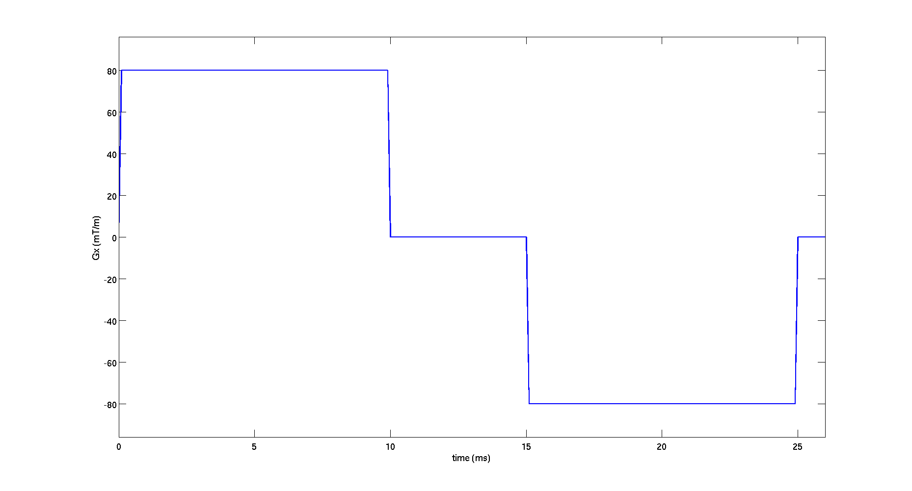
View the first waveform in the protocol

The previous diffusion protocol has 30 measurements with varying timing parameters and number of oscillations. To visualize the gradient waveform for the first measurement, run the following code:

figure();
Gx = protocolGEN.G(1,1:3:end);
plot((0:tau:(length(Gx)-1)*tau)*1E3,Gx*1000,'LineWidth',2)
xlim([0,(protocolGEN.smalldel(1)+protocolGEN.delta(1)+10*tau)*1E3])
ylim([min(Gx)*1200 max(Gx)*1200])
xlabel('time (ms)','FontSize',16);
ylabel('Gx (mT/m)','FontSize',16);
set(gca,'FontSize',16);

Synthesize the diffusion signal for this protocol

In order to synthesize diffusion signal, we need to choose a diffusion substrate.

Chose a white-matter model:

model.name = 'ZeppelinCylinder';
di = 1.7E-9; % intrinsic diffusivity
dh = 1.2E-9; % hindered diffusivity
rad = 4E-6; % cylinder radius
% angles in spherical coordinates describing the cylinder orientation; 
theta = 0; % angle from z axis
phi = 0; % azimuthal angle
ficvf = 0.7; % intracellular volume fraction
model.params = [ficvf di dh rad theta phi];

Add the matrices and other constants required by the Matrix Method:

protocolGEN = MMConstants(model,protocolGEN);

Compute the diffusion signal for the given protocol and model. The signal is a 30x1 vector containing the results for each measurement.

signal = SynthMeas(model,protocolGEN);

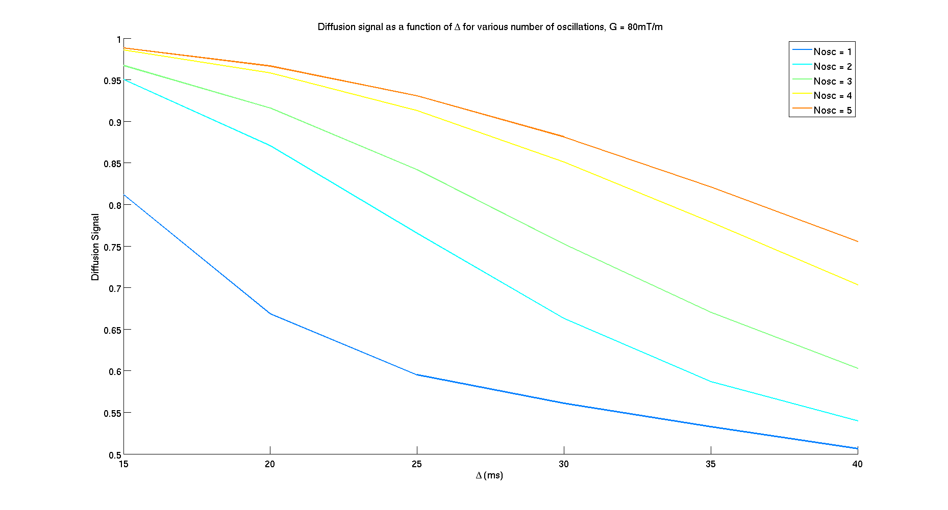
Plot the synthesized diffusion signal

To visualize the diffusion signal computed in the previous step as a function of diffusion time, run the following code:

signal_matrix = reshape(signal,length(Nosc),length(delta));
figure();
colors = jet(length(Nosc));
hold on;
for i  = 1:length(Nosc)  
    legend_name{i} = ['Nosc = ' num2str(Nosc(i))];
    plot(delta*1000,signal_matrix(i,:),'LineWidth',2,'Color',colors(i,:));
end
xlabel('\Delta (ms)','FontSize',16);
ylabel('Diffusion Signal','FontSize',16);
set(gca,'FontSize',16);
title('Diffusion signal as a function of \Delta for various number of oscillations, G = 80mT/m')
legend(legend_name,'FontSize',16)

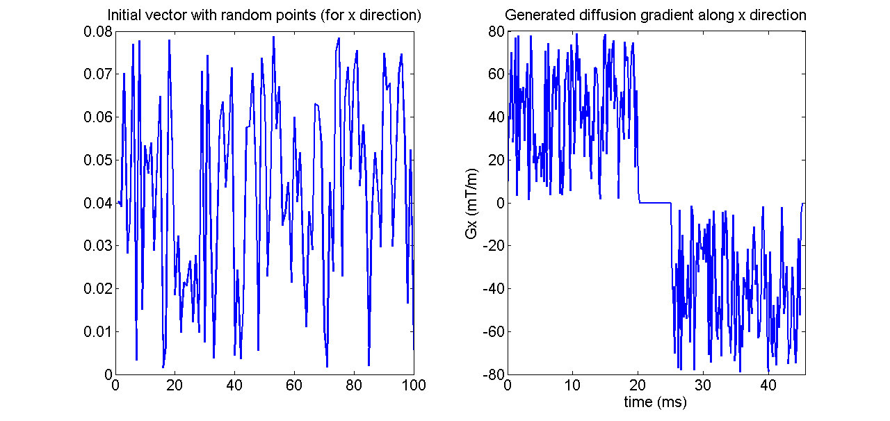
Example 2: random gradient waveform. To show the true potential of MISST which can work with any diffusion sequence, for this example we chose a diffusion gradient given by 3 vectors of random numbers for gradients in x,y and z directions.

Here you will see how to create a valid gradient waveform from a 3 vectors which specifies the value of the gradient at each point in time in x, y and z directions.

Create the protocol needed for the diffusion simulation:

clear all
smalldel = 0.02; % duration of the waveform;
Npoints = 100; % 100 random points
tau = smalldel / Npoints; % sampling interval
p180 = 0.005; % time interval between the first and second waveforms (duration of rf pulse)
Gmax = 0.08; % maximum gradient in T/m;
% the gradient waveform will be repeated after the 180 pulse
wf = [rand(1,Npoints)*Gmax; rand(1,Npoints)*Gmax; rand(1,Npoints)*Gmax]; 
% gradient waveform consists of random points along x, y and z  
% create protocolGEN in the necessary format
protocolGEN.G = [zeros(1,3) wf(:)' zeros(1,3* round(p180/tau)) -wf(:)' zeros(1,3)]; 
protocolGEN.tau=tau;
protocolGEN.pulseseq = 'GEN';

View the gradient along x direction. Gradients along y and z look similar.

 figure();
subplot(1,2,1)
plot(wf(1,:),'LineWidth',2)
title('Initial vector with random points (for x direction)','FontSize',16);
set(gca,'FontSize',16);
subplot(1,2,2)
Gx = protocolGEN.G(1,1:3:end);
plot((0:protocolGEN.tau:(length(Gx)-1)*protocolGEN.tau)*1E3,Gx*1000,'LineWidth',2)
xlabel('time (ms)','FontSize',16);
ylabel('Gx (mT/m)','FontSize',16);
title('Generated diffusion gradient along x direction','FontSize',16);
set(gca,'FontSize',16);
xlim([0,(length(Gx)+1)*tau*1E3])

Choose the diffusion substrate (same as before)

model.name = 'ZeppelinCylinder';
di = 1.7E-9; % intrinsic diffusivity
dh = 1.2E-9; % hindered diffusivity
rad = 4E-6; % cylinder radius
% angles in spherical coordinates describing the cylinder orientation; 
theta = 0; % angle from z axis
phi = 0; % azimuthal angle
ficvf = 0.7; % intracellular volume fraction
model.params = [ficvf di dh rad theta phi];

Add the matrices and other constants required by the Matrix Method:

protocolGEN = MMConstants(model,protocolGEN);

Compute the diffusion signal for the given protocol and model:

signal = SynthMeas(model,protocolGEN);

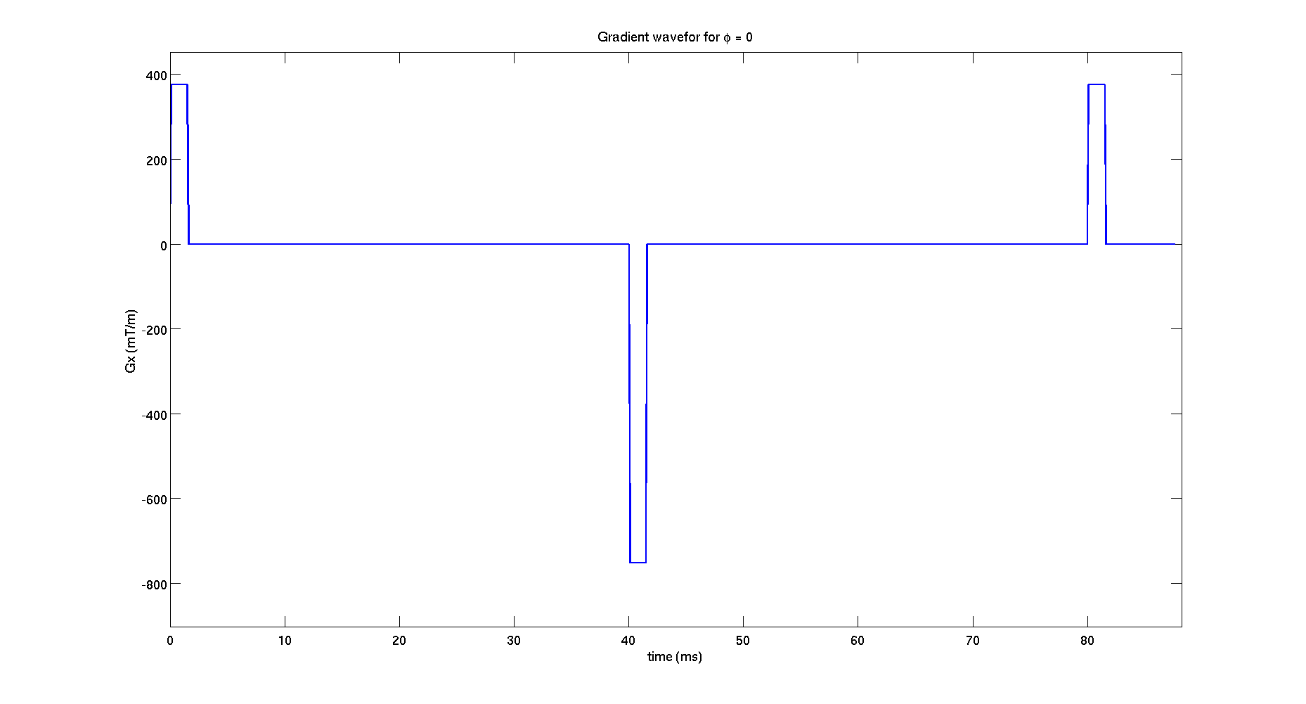
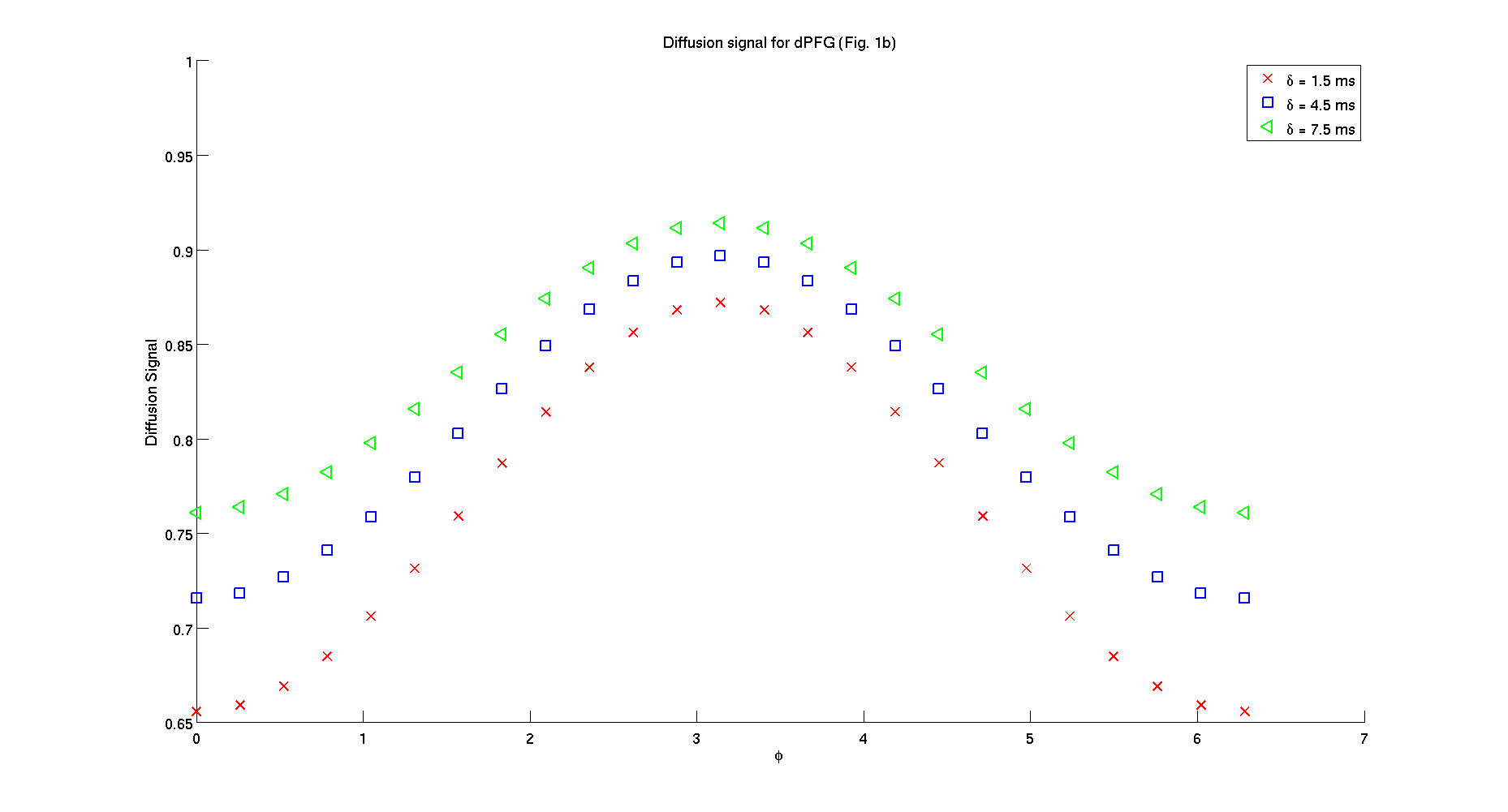
Example 3: diffusion sequences used in Drobnjak et al. 2011 .
1. dPFG sequences for parameters used in Figure 1b from Drobnjak et al. 2011.

Create the dPFG protocol with the same parameters as in Drobnjak et al 2011:

 clear all 
Npoints = 25;
protocoldPFG1.pulseseq = 'dPFG';
protocoldPFG1.smalldel = [repmat(0.0015,1,Npoints) repmat(0.0045,1,Npoints) ...
      repmat(0.0075,1,Npoints)];
protocoldPFG1.G = [repmat(0.3757,1,Npoints) repmat(0.1252,1,Npoints) ...
      repmat(0.0751,1,Npoints)]; 
protocoldPFG1.delta = repmat(0.04,1,Npoints*3);
protocoldPFG1.theta = repmat(pi/2,1,Npoints*3);
protocoldPFG1.phi = repmat(0,1,Npoints*3); % first gradient along x direction
protocoldPFG1.theta1 = repmat(pi/2,1,Npoints*3);
% second gradient rotating in x-y plane
protocoldPFG1.phi1 = repmat(linspace(0,2*pi,Npoints),1,3); 
protocoldPFG1.tm = repmat(0,1,Npoints*3);
tau = 1E-4;
protocoldPFG1.tau = tau;

Create the GEN protocol:

protocolGEN.pulseseq = 'GEN';
protocolGEN.G = wave_form(protocoldPFG1);
protocolGEN.tau = tau;

Display the gradient waveform along x direction for the first pulse sequence:

figure();
G_plot = protocolGEN.G(1,1:3:end);
plot((0:tau:(length(G_plot)-1)*tau)*1E3,G_plot*1000,'LineWidth',2)
 xlim([0,(length(G_plot)+5)*tau*1E3])
 ylim([min(G_plot)*1200 max(G_plot)*1200])
 set(gca,'FontSize',16);
 xlabel('time (ms)','FontSize',16);
 ylabel('Gx (mT/m)','FontSize',16);
 title('Gradient wavefor for \phi = 0')

Add tissue model

model.name = 'Cylinder';
di = 2E-9; % intrinsic diffusivity
rad = 5.2E-6; % cylinder radius
% angles in spherical coordinates describing the cylinder orientation; 
theta = 0; % angle from z axis
phi = 0; % azimuthal angle
model.params = [ di rad theta phi];

Add the matrices and other constants necessary for the matrix method

protocolGEN = MMConstants(model,protocolGEN);

Compute diffusion signal for the given protocol and model

signal = SynthMeas(model,protocolGEN);

Plot the diffusion signal as a function of the angle between the two gradients (Fig. 1b)

 signal_plot = reshape(signal,Npoints,3);
figure();
hold on;  
plot(linspace(0,2*pi,Npoints),signal_plot(:,1),'xr',...
    linspace(0,2*pi,Npoints),signal_plot(:,2),'sb',...
    linspace(0,2*pi,Npoints),signal_plot(:,3),'<g',...
    'LineWidth',2,'MarkerSize',12);
xlabel('\phi','FontSize',16);
ylabel('Diffusion Signal','FontSize',16);
legend('\delta = 1.5 ms','\delta = 4.5 ms','\delta = 7.5 ms')
set(gca,'FontSize',16);
title('Diffusion signal for dPFG (Fig. 1b)')

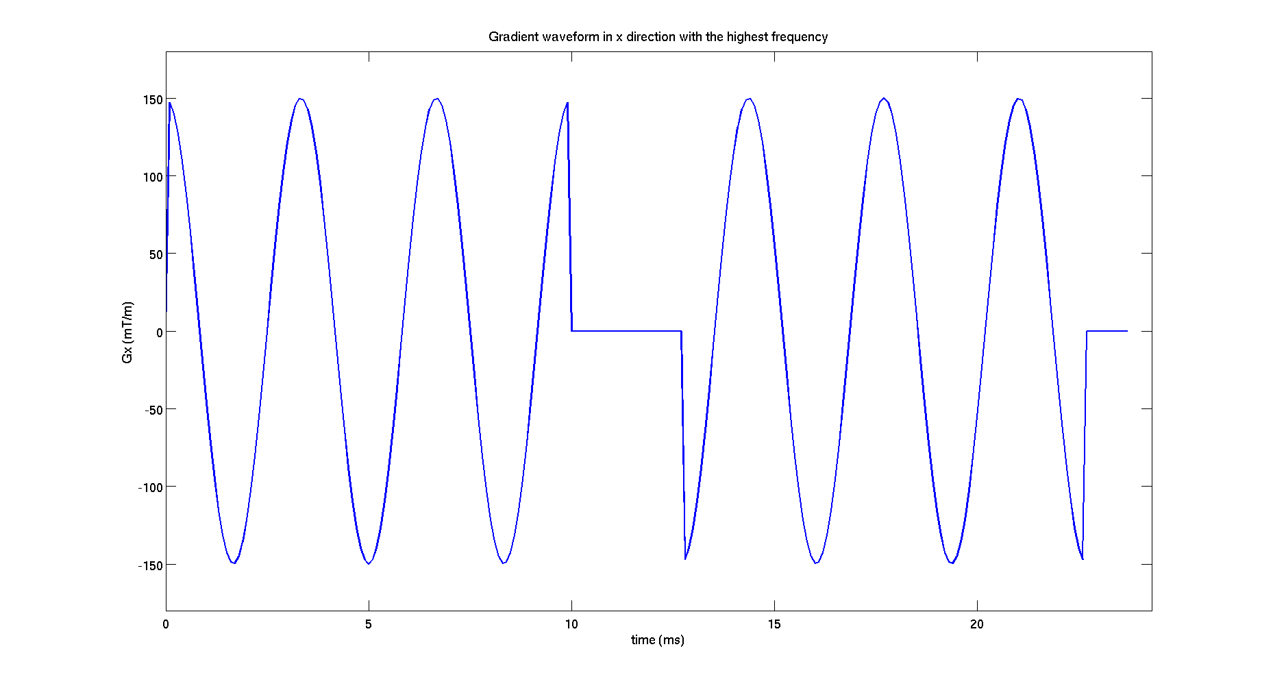
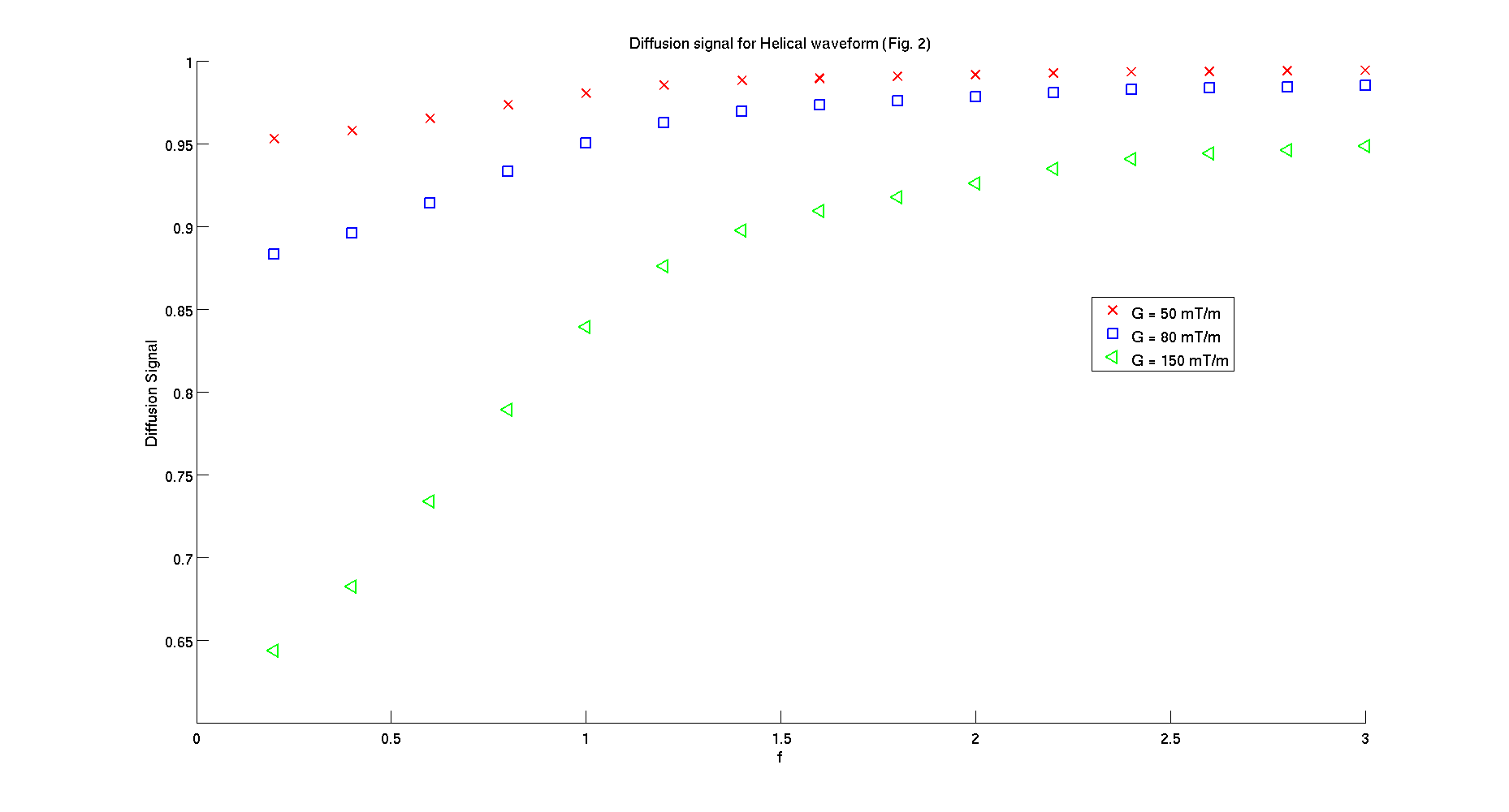
2. Helical waveforms for parameters used in Figure 2b from Drobnjak et al. 2011.

Create the helical waveform protocol with the same parameters as in Drobnjak et al 2011:

 clear all
fosc = 0.2:0.2:3; % normalized frequency
smalldel = 0.01; % duration
delta = 0.0127;
protocolHelical.pulseseq = 'Helical';
protocolHelical.smalldel = repmat(smalldel,1,length(fosc)*3) ;
protocolHelical.G = [repmat(0.05,1,length(fosc)) repmat(0.08,1,length(fosc))...
       repmat(0.15,1,length(fosc))];
protocolHelical.delta = repmat(delta,1,length(fosc)*3);
protocolHelical.omega = repmat(2*pi*fosc/smalldel,1,3);
protocolHelical.slopez = repmat(1/5/smalldel,1,length(fosc)*3);
tau = 1E-4;
protocolHelical.tau = tau;

Create the GEN protocol:

protocolGEN.pulseseq = 'GEN';
protocolGEN.G = wave_form(protocolHelical);
protocolGEN.tau = tau;

Plot the gradient waveform with the highest frequency

figure();
G_plot = protocolGEN.G(end,1:3:end);
plot((0:tau:(length(G_plot)-1)*tau)*1E3,G_plot*1000,'LineWidth',2)
 xlim([0,(length(G_plot)+5)*tau*1E3])
 ylim([min(G_plot)*1200 max(G_plot)*1200])
 xlabel('time (ms)','FontSize',16);
 ylabel('Gx (mT/m)','FontSize',16);
 set(gca,'FontSize',16);
 title('Gradient waveform in x direction with the highest frequency','FontSize',16);

Add the tissue model

model.name = 'Cylinder';
di = 2E-9; % intrinsic diffusivity
rad = 5E-6; % cylinder radius
% angles in spherical coordinates describing the cylinder orientation; 
theta = 0; % angle from z axis
phi = 0; % azimuthal angle
model.params = [ di rad theta phi];

Add the matrices and other constants necessary for the matrix method

protocolGEN = MMConstants(model,protocolGEN);

Compute diffusion signal for the given protocol and model

signal = SynthMeas(model,protocolGEN);

Plot the diffusion signal as a function of the normalized frequency (Fig 2b)

signal_plot = reshape(signal,length(fosc),3);
figure();
hold on;  
plot(fosc,signal_plot(:,1),'xr',...
    fosc,signal_plot(:,2),'sb',...
    fosc,signal_plot(:,3),'<g',...   
    'LineWidth',2,'MarkerSize',12);
xlabel('f','FontSize',16);
ylabel('Diffusion Signal','FontSize',16);
legend('G = 50 mT/m','G = 80 mT/m','G = 150 mT/m')
set(gca,'FontSize',16);
title('Diffusion signal for Helical waveform (Fig. 2b)')

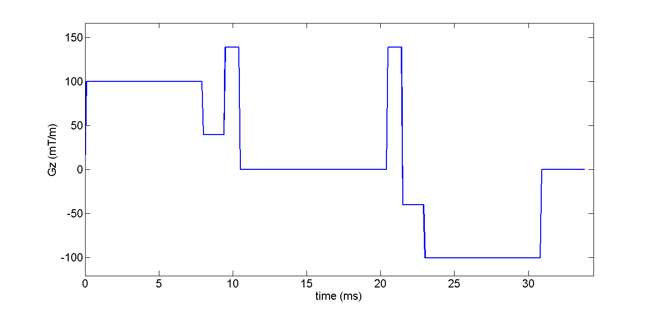
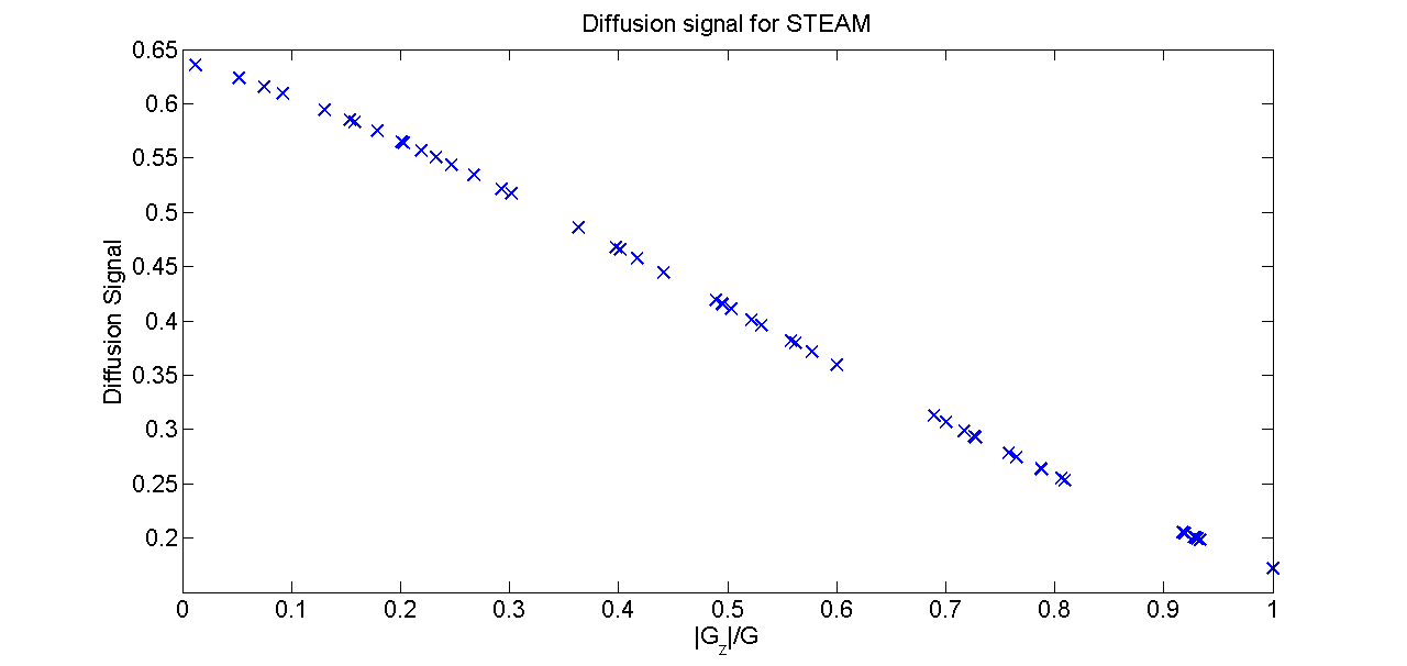
3. STEAM sequences for parameters used in Figure 3b from Drobnjak et al. 2011.

Create the STEAM protocol with the same parameters as in Drobnjak et al 2011:

clear all
protocolSTEAM.pulseseq = 'STEAM';
protocolSTEAM.smalldel = repmat(0.0079,1,50);
protocolSTEAM.sdels = repmat(0.001,1,50);
protocolSTEAM.sdelc = repmat(0.0015,1,50);
protocolSTEAM.G = repmat(0.14,1,50);
protocolSTEAM.Gs = repmat(0.139,1,50);
protocolSTEAM.Gc = repmat(0.04,1,50);
protocolSTEAM.grad_dirs = abs(ReadCaminoElecPS(sprintf('PointSets/Elec%03i.txt',50)));
protocolSTEAM.tau1 = repmat(0,1,50);
protocolSTEAM.tau2 = repmat(0,1,50);
protocolSTEAM.tm = repmat(0.01,1,50);
tau = 1E-4;
protocolSTEAM.tau = tau;

Create the GEN protocol:

protocolGEN.pulseseq = 'GEN';
protocolGEN.G = wave_form(protocolSTEAM);
protocolGEN.tau = tau;

Plot the gradient waveform in z direction for the measurement

figure();
Gz = protocolGEN.G(1,3:3:end);
plot((0:tau:(length(Gz)-1)*tau)*1E3,Gz*1000,'LineWidth',2)
 xlim([0,(length(Gz)+5)*tau*1E3])
 ylim([min(Gz)*1200 max(Gz)*1200])
 xlabel('time (ms)','FontSize',16);
 ylabel('Gz (mT/m)','FontSize',16);
 set(gca,'FontSize',16);

Add the tissue model

model.name = 'Cylinder';
di = 0.7E-9; % intrinsic diffusivity
rad = 5E-6; % cylinder radius
% angles in spherical coordinates describing the cylinder orientation; 
theta = 0; % angle from z axis
phi = 0; % azimuthal angle
model.params = [ di rad theta phi];

Add the matrices and other constants necessary for the matrix method

protocolGEN = MMConstants(model,protocolGEN);

Compute diffusion signal for the given protocol and model

signal = SynthMeas(model,protocolGEN);

Plot the diffusion signal as a function of |Gz|/G (Fig 3b)

signal_plot = signal;
Gplot = abs(protocolSTEAM.grad_dirs(:,3));
figure();
plot(Gplot,signal_plot,'x','LineWidth',2,'MarkerSize',12);
xlabel('|G_z|/G','FontSize',16);
ylabel('Diffusion Signal','FontSize',16);
set(gca,'FontSize',16);
title('Diffusion signal for STEAM Fig. 3b')

To help you start, the same commands are part of the scripts in the folder MISST/example

MISST tutorials

Understand the format of the gradient waveform necessary for the simulation:

The information about the diffusion protocol is passed to the simulator as the fields of a Matab structure, which we conveniently call "protocol" in the examples. To generate the diffusion signal for a discrete generalized waveform, the structure protocol should have the following fields:

protocol.pulseseq = 'GEN' - the name of the sequence, -->protocol.G - discrete gradient waveforms which contain the gradient components (Gx , Gy and Gz ) at each point in time from the beginning of the measurement until the readout

protocol.tau - time interval between two points on the gradient waveform

Optional:

protocol.smalldel - gradient duration

protocol.delta - time interval between the onset of the first and second pulse.

It is not mandatory to specify the last two parameters, but they save computation time if the diffusion sequence has two gradient intervals. Additionally the user can specify if the second gradient is repeated protocol.mirror = 0 (default value) or reflected protocol.mirror = 1 .

The gradient waveform protocol.G is a M x 3K matrix which stores the values of the diffusion gradient at each time point. Each row represents one measurement and contains the values of the gradients in x, y and z direction. M is the total number of measurements and K is the number of gradient points in each direction for one measurement:

G1x(1) G1y(1) G1z(1) G1x(2) G1y(2) G1z(2) ... G1x(K) G1y(K) G1z(K)

G2x(1) G2y(1) G2z(1) G2x(2) G2y(2) G2z(2) ... G2x(K) G2y(K) G2z(K)

...

GMx(1) GMy(1) GMz(1) GMx(2) GMy(2) GMz(2) ... GMx(K) GMy(K) GMz(K)

protocol.G includes the complete diffusion gradient and the user should take into account any realistic situations such as the duration of the rf pulses, crusher gradients, etc.

protocol.G should satisfy the echo condition, that the integral of the gradient over time should be 0.

Understand the tissue models available in the simulation:

MISST uses the 3D extension of the Matrix Method (first introduced by Callaghan JMR 95) presented in Drobnjak et al 2011. For the diffusion substrates, we follow the naming scheme presented in Panagiotaki et al. 2012. The following substrates are available in MISST:

Basic compartments with Gaussian diffusion:

Ball (isotropic free diffusion)

Zeppelin (anisotropic, cylindrically symmetric diffusion tensor)

Tensor (full diffusion tensor)

Basic compartments with restricted diffusion:

Stick

AstroSticks (isotropically oriented sticks)

Cylinder

AstroCylinders (isotropically oriented cylinders)

Sphere

Dot (fully restricted)

Multi-compartment models:

ZeppelinCylinder

TortZeppelinCylinder (same as ZeppelinCylinder, but with tortuosity constraint on volume fraction)

TortZeppelinCylinderBall

Other substrates can be easily implemented by the user once familiarized with the code.

All the information related to the diffusion substrate is stored in a MATLAB structure, which we call “model” in the examples. For the purpose of signal generation, “model” has only two fields: model.name – the name of the model (listed above) and model.params - the values of the model parameters in S.I. units (m, s, etc.) of each model. See documentation for details.